


Serviços Personalizados
artigo
 Inglês (pdf)
 Artigo em XML
 Referências do artigo
Indicadores

Compartilhar

 Permalink
Journal of Human Growth and Development
versão impressa ISSN 0104-1282versão On-line ISSN 2175-3598
J. Hum. Growth Dev. vol.28 no.3 São Paulo set./dez. 2018
http://dx.doi.org/10.7322/jhgd.152180
ORIGINAL ARTICLE
Complex measurements of heart rate variability in obese youths: distinguishing autonomic dysfunction
David M. GarnerI; Franciele Marques VanderleiII; Luiz Carlos Marques VanderleiIII
ICardiorespiratory Research Group, Department of Biological and Medical Sciences,Faculty of Health and Life Sciences, Oxford Brookes University, Headington Campus, Gipsy Lane, Oxford OX3 0BP, United Kingdom
IIDepartment of Physiotherapy, UNESP - Univ Estadual Paulista - Presidente Prudente, São Paulo, Brazil
IIIDepartment of Physiotherapy, UNESP - Univ Estadual Paulista - Presidente Prudente, São Paulo, Brazil
ABSTRACT
INTRODUCTION: Heart rate variability (HRV) can be assessed from RR-intervals. These are derived from an electrocardiographic PQRST-signature and can deviate in a chaotic or irregular manner. In the past, techniques from statistical physics have allowed researchers to study such systems
OBJECTIVE: This study planned to assess the heart rate dynamics in young obese subjects by nonlinear metrics to heart rate variability
METHOD: 86 subjects were split equally according to status. Heart rate was recorded with the subjects resting in a dorsal (prone) position for 30 minutes. The complexity of the RR-intervals was assessed by five Entropies, Detrended Fluctuation Analysis, Higuchi and Katz's fractal dimensions Following inconclusive tests of normality we calculated the One-Way Analysis of Variance, Kruskal-Wallis, and the Effect Sizes by Cohen's d significances
RESULTS: It was established that Shannon, Renyi and Tsallis Entropies and the Higuchi and Katz's fractal dimensions could significantly discriminate the two groups. The three entropies were higher in obese youths, suggesting less predictable sets of RR intervals (p<0.0001; d≈1.0). Whilst the Higuchi (p<0.003; d≈0.76) and Katz's (p≈0.02; d≈0.57) fractal dimensions were lower in obese youths
CONCLUSION: As with chaotic globals an increase in response was detected by three measures of entropy in young obese. This is counter to the decreasing response detected by fractal dimensions. Chaotic globals and entropies are more dependable than fractal dimensions when assessing the responses to obesity
Keywords: youth obesity, detrended fluctuation analysis, entropy, fractal dimensions
INTRODUCTION
Heart rate variability (HRV) can be assessed from RR-intervals1,2. These are derived from an electrocardiographic PQRST-signature and can deviate in a chaotic or irregular manner. In the past, techniques from statistical physics3,4 have allowed researchers to study such systems5.
HRV is an inexpensive, reliable and non-invasive technique to monitor the sympathetic and parasympathetic components of the autonomic nervous system (ANS)6. HRV is highly regarded as a functional marker of human development7. It can be enforced to identify phenomena related to the ANS in healthy subjects and patients with certain diseases, such as diabetes mellitus8, 9, chronic obstructive pulmonary disorder (COPD)10, epilepsy11,12 and those referred to as "dynamical diseases13."
Previously, we have assessed datasets through chaotic globals in obese youths14. These techniques are useful since they can be applied straightforwardly to entire and in particular short time-series (20 minutes) to achieve statistically significant responses. So far, these techniques are formulated by enforcing either Welch15 or Multi-Taper Method16,17 (MTM) power spectra, so the phase information is lost. This provides the motivation to assess these datasets of obese youths by alternative complex measures. In this study we enforce five based on entropy: Approximate18, Sample19,20, Shannon21, Renyi22,23 and Tsallis24 Entropies and then, the Detrended Fluctuation Analysis (DFA)25. Furthermore, we then assessed the same data using the Higuchi26 and Katz's27 fractal dimensions.
METHODS & STATISTICAL ANALYSES
Patient Selection and assessments were exactly as the study by Vanderlei et al14.
Shannon entropy
Shannon Entropy21 is a measure of lack of knowledge. A low entropy dataset is highly predictable - whereas a high entropy dataset is less predictable. In contrast to Tsallis and Renyi entropies (discussed next), Shannon entropy is additive. Hence, if the probabilities can be factorised into independent factors, the entropy of the joint process is the sum of the entropies of the separate processes.
Renyi entropy
The order-q Renyi entropies22 are a series of entropy like quantities. When the entropic order α→ 1, Renyi entropy coincides with Shannon entropy; which can be derived by the l'Hospital's rule28,29. Here we set the entropic order α=0.25. As entropic order increases the measures become more sensitive to the values occurring at higher probabilities and less to those of lower probabilities. Renyi entropy is described fully in studies by Zyczkowski23.
Tsallis entropy
Tsallis entropy24 is a generalisation of the standard Shannon-Boltzmann-Gibbs entropy. It was introduced as a basis for generalising the standard statistical mechanics. Where entropic index, q →1 it is the Shannon-Boltzmann-Gibbs entropy. Here we set entropic index, q=0.25. Tsallis entropy is discussed further in the publications by dos Santos30 and, Plastino and Plastino31.
Detrended fluctuation analysis (DFA)
DFA25 can be applied to datasets where statistics such as mean, variance and autocorrelation vary with time. DFA is a technique quantifying how the fluctuations of a signal scale with the number of samples of that signal. Regarding DFA according to Donaldson32 the time-series of length k was manipulated as follows.

The integrated time-series was then divided into equally sized and non overlapping windows of length w. A linear regression line was fitted through the data in each window and the time-series manipulated by subtracting the regression line from the data. The root mean square fluctuation F(w) of the integrated and detrended time-series defined as
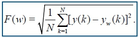
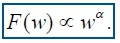
The scaling exponent is obtained as the slope of the straight line fit to F(w) against w on a log-log plot as:
DFA is a widely enforced technique in variability analysis. It has been applied to the evaluation of posture33, exercise34, sleep stages35, prediction of sepsis36, classification of asthma37 and COPD32,38,39.
Approximate entropy (apen)
ApEn18, is a procedure necessary to assess the level of regularity and the unpredictability of changes over time-series. ApEn is the logarithmic ratio of component-wise matching sequences from the signal length, N. Other parameters include r, tolerance and m the embedding dimension. Here, we set m to 2 and r is 0.2 of the standard deviation of the data.
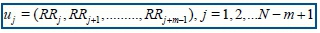
A minimum value of zero for ApEn would indicate a totally predictable series. ApEn is described mathematically as in the Kubios HRV® Analysis Manual40. First a set of length m vectors uj is formed
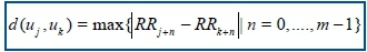
The distance between these vectors is defined as the maximum absolute difference between the corresponding elements, hence,
Next for each uj the relative number of vectors uk for which (uj, uk) is calculated. This index is denoted with and can be written in the form
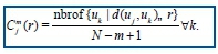
Due to the normalisation, the value of Cmj(r) is always smaller or equal to 1. Note that the value is at least 1/(N - m + 1) since uj is also included in the count. Then, take the natural logarithm of each Cmj(r) and average over j to yield.
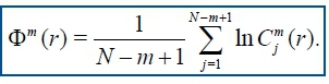
Finally, the ApEn is obtained as

Sample entropy (SampEn)
SampEn19,40 is analogous to ApEn but there are two important differences in its calculation. For ApEn, in the calculation of the number of vectors uk for which (uj, uk), r, also the vector uj itself is included. This ensures that Cmj(r) is always larger than zero and the logarithm can be applied, but at the same time it makes ApEn biased. In SampEn, the self-comparison of uj is eliminated by calculating Cmj(r) as
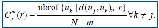
Now the value of Cmj(r) will be between 0 and 1. Then, the values of Cmj(r) are averaged to yield:
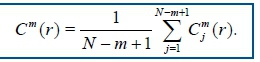
SampEn isdeduced as

Again, the embedding dimension is m and the tolerance parameter r (where, m=2 and r=0.2 of the standard deviation of the data). Both ApEn and SampEn are estimates for the negative natural logarithm of the conditional probability that a data of length N, having repeated itself within a tolerance r for m points will also repeat itself for m+1 points.
Higuchi fractal dimension (HFD)
Higuchi26 derived his procedure to measure the fractal dimension of discrete time sequences. It is regarded as the most robust of all the fractal dimension techniques and can be enforced on relatively short sections of data. It is imposed directly to the RR-intervals with no power spectrum step as is the case with the chaotic globals8, 9. The phase information is maintained.
Khoa et al41 presented the algorithm and we adapt it below for RR intervals. It is based on a measure of length, L(k), of the curve that represents the considered time-series while using a segment of k samples as a unit, if L(k) scales in the following manner:
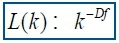
The curve is alleged to display a fractal dimension Df. A simple curve has dimension equal to 1 and a plane has dimension equal to 2. The value of Df is always between 1 (a simple curve) and 2 (a curve which almost fills out the whole plane). Df quantifies the complexity of the curve and so of the time-series this curve represents on a graph.
From a given time series, RR(1), RR(2), ... , RR(N), the algorithm constructs k new time series:
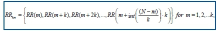
Where m is initial time value, k indicates the discrete time interval between points, hence the delay, kmax is maximum interval time, int(a) is integer part of a real number a.
For each of the time-series RRkm constructed, the average length Lm (k) is then computed as:
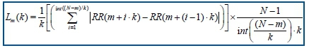
N is total number of RR intervals. Subsequently, the length of the curve for time interval k is expressed as the sum value over k sets of Lm (k) as illustrated by the following equation.

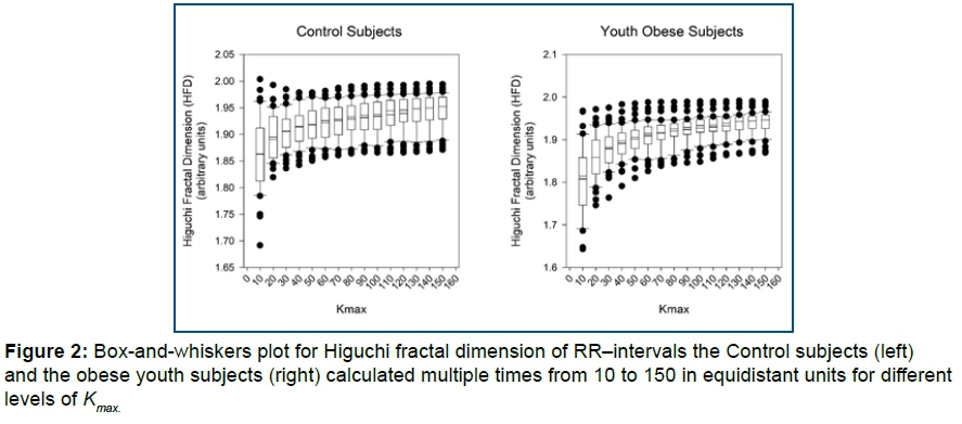
Lastly, the slope of the curve 1n(L(k)) /1n(1 /k) is estimated using least squares linear best fit and the resulting slope is the HFD. To select a suitable value for kmax, HFD values are plotted against a range of kmax. The point at which the fractal dimension plateaus is considered a saturation point. That appropriate kmax value should be selected.
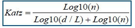
Katz's fractal dimension
Regarding the Katz's algorithm27 this fractal dimension is once more calculated directly from the time-series. This algorithm has the advantage over that of Higuchi's in that a kmax parameter is superfluous. Yet, it has the difficulty that it requires a longer time-series to achieve significant results. Therefore we apply a cubic spline interpolation42 at levels 1 Hz to 15 Hz. As a consequence the number of samples in the datasets increases by 1000 per 1 Hz increase. It is important to recall that an accurate value for any type of fractal dimension should be between 1 and 2, as stated in the preceding section (see results later).
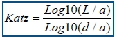
L is the total length of the time-series and d is the Euclidean distance between the first point in the series and the point that provides the furthest distance with respect to this first point. If we set a to be the mean distance between successive points and, n as the number of steps in the curve, then n = L/a.
RESULTS
Parametric statistics recognize that the relevant datasets are normally distributed, hence the use of the mean as a measure of central tendancy. If we cannot normalize the data it is unsuitable to compare means. To authenticate normality we executed the Anderson-Darling43 and Ryan-Joiner44 tests. Unfortunately, the results were inconclusive so we are unable to assert that the observations follow either a normal or non-normal distribution. Thus, we applied both parametric and non-parametric tests of significance. These are the One-Way Analysis of Variance (ANOVA1)45 and the Kruskal-Wallis46 tests of significance.
To quantify the magnitude of difference between protocols for significant differences, the effect size was calculated via Cohen's d47. Large effect size was considered for values greater than or equal to 0.9, medium for values between 0.9 and 0.5 and small for values between 0.5 and 0.25.
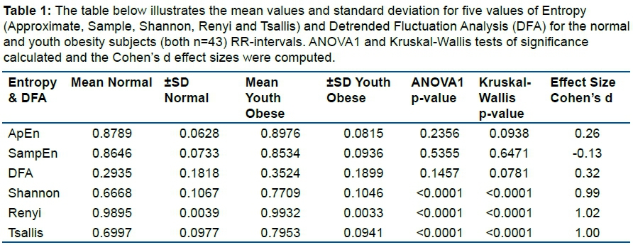
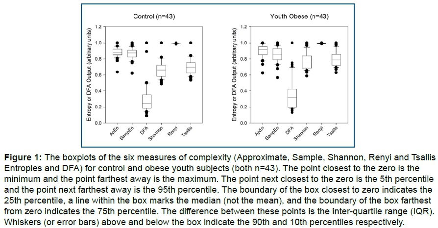
The results reveal extensive variation for both the non-obese controls and those from the obese youths (see Table 1 and Figure 1). The results for the Approximate Entropy, Sample Entropy and DFA are insignificant and so are not discussed further. The results for Shannon, Renyi and Tsallis entropy are all highly significant on the basis of all three statistical tests (p<0.0001 & Cohen's d ≈ 1.0 large effect size). In all three cases there is a significant increase in chaotic response.
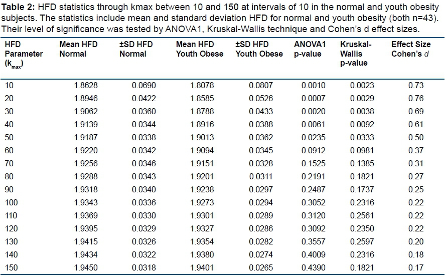
Next, we assessed the HFD there were several significant results at numerous levels of kmax. These values of kmax were between 10 and 50 and all achieved a p<0.05 (<5%) and a Cohen's d effect size of d > 0.5, a medium effect size. However, the algorithm performed optimally with a kmax of 20 (ANOVA1 and Cohen's d). This was related to a decrease in mean values for HFD from normal non-obese to obese youths. This was assumed to be the saturation point. During the HFD analysis exactly 1000 RR intervals from the two groups was enforced.
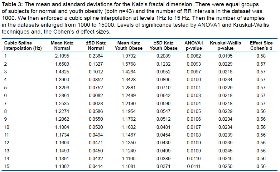
Unlike HFD the Katz's algorithm necessitates a longer time-series. Accordingly, we enforced a cubic spline interpolation42 at levels 1 Hz to 15 Hz. As a consequence the number of samples in the datasets enlarged from 1000 to 15000 increasing by 1000 per single 1 Hz increase.
It should be emphasized that with a cubic spline interpolation of 1Hz (the original time-series) the results were erroneous because they gave a value of Katz's fractal dimensions greater that 2. This is inappropriate as all fractal dimesions are required to be between 1 (simple curve) and 2. (curve almost filling entire plane) This is error is assumed to be attributable to the too shorter time series.
There was an optimal level of significance with a decrease in mean values from normal non-obese to youth obese for the Katz's algorithm (p≈0.02; ≈2% both ANOVA1 & Kruskal-Wallis tests) and a medium effect size (Cohen's d≈0.57) for a cubic spline interpolation of 2 Hz. With longer time-series and cubic spline interpolations greater than 2Hz the significances of the results gradually decline for all three statistical tests.
DISCUSSION
The development of algorithms to function as statistical markers of pathological disease states is an ongoing process. This is particularly the case with the measurements based on RR-intervals by non-linear dynamics and their relationship with the "dynamical diseases." Time and frequency domain or geometric methods can incorrectly interpret the level of pathology.
Previously when employing short-time series for the assessment of chaotic response in youth obese subjects we have computed the chaotic global techniques to discriminate between control subjects and those obese youths14. Generally, these chaotic global techniques are sufficient. However, during the power spectral step through Welch or MTM, the phase information is lost. This was the motivation to apply the same data to other techniques based on nonlinear dynamics. There were five entropies, DFA and two categories of fractal dimension. Here the phase information is preserved and they are less computer processor expensive.
The responses of Approximate and Sample Entropies and DFA are insignificant. However, by applying Shannon, Renyi and Tsallis Entropies a significant increase in values for obese youths was observed, suggesting that the series of RR intervals in these individuals is less predictable. There was a slight statistical advantage for the Renyi Entropy over Shannon and Tsallis when assessed by effect size Cohen's d with the entropic order α=0.25. But, they were largely similar on ANOVA1 and Kruskal-Wallis statistical tests.
In a preceding study by Vanderlei et al48 with obese children a similar connection was found. But, the previous study with obese children48 found that Approximate Entropy was also significant (p<0.01, <1%). Further, in this study we calculated DFA and this was also established statistically insignificant.
In relation the HFD (p<0.003, p≈0.3%; d≈0.76 medium effect size) was revealed to be superior to the Katz's fractal dimension (p≈0.02, p≈2%; d≈0.57 medium effect size) when the ANOVA1, Kruskal-Wallis and Cohen's d tests were computed. These were both significant decreases in chaotic response by Higuchi and Katz's fractal dimension of HRV in obese youth subjects. The decreases in chaotic response attributable to the fractal dimensions are uncharacteristic.
Some chaotic global (including CFP1, CFP3 and CFP6)14 and the Shannon, Renyi and Tsallis Entropies (see Table 1 and Figure 1 above) have been revealed to increase in magnitude for the obese youths using the identical dataset14. Besides, when applied to obese children the most robust chaotic global (CFP1; with p≈0.05;49) and four out of five measures of entropy, not the Sample Entropy (p>0.05)48 significantly increased in obese children. Interestingly, in a study of malnourished children50 the chaotic global parameters (CFP1 & CFP3) significantly decreased, the opposite response to obesity in children or obese youths; excluding consideration of the two fractal dimensions. It could therefore be assumed that whilst the fractal dimension techniques described here discriminate between the two cohorts of data they cannot be used effectively or reliably as a statistical marker for youth obesity. It is advisable that in this case the chaotic globals or three entropic techniques are unmatched.
The relationship between youth obesity and complexity measures such as chaotic globals and the three entropies (Shannon, Renyi and Tsallis) is beneficial in the risk assessment of diseases associated with obesity. Through non-invasive technology it identifies the level of severity from a low-cost yet reliable method of monitoring the ANS. This is helpful in treatments, such as the determination of the extent of dietary or pharmacological interventions required in the purported "dynamical diseases."
Yet, proceeding cautiously, since the subject's autonomic modulation may be critical. It should be highlighted that malnutrition by large has the opposite effect on the chaotic responses of RR-intervals to chaotic globals and entropies, excluding the two fractal dimensions; Higuchi and Katz's. Also, it should be distinguished that there are other conditions, such as diabetes mellitus and COPD which could cause similar correlations.
CONCLUSION
On the basis of three measurements of non-linearity, namely Shannon, Renyi and Tsallis Entropy young obese subjects have exhibited an increase suggesting a series of RR intervals that are less predictable. It was revealed that both Higuchi and Katz’s fractal dimension can discriminate between the two groups. The Higuchi fractal dimension was optimal with a kmax of 20 and with 1000 samples. For the Katz’s Fractal Dimension the maximal discrimination between the groups necessitated a cubic spline interpolation of 2Hz and therefore 2000 samples. Yet these fractal dimension techniques lead to a decrease in chaotic response when comparing normal non-obese to obese youths. This is atypical. So it is advisable to enforce chaotic globals or the three named entropies as a statistical marker for obesity as they are more consistent.
Competing interests
The authors declare that there is no conflict of interests regarding the publication of this article
Acknowledgements
The authors are grateful to CNPq (National Council of Scientific and Technological Development) financial support for this study (Proc. n° 307361/2011-0).
REFERENCES
1.Goldberger AL. Cardiac chaos. Science. 1989;243(4897):1419. [ Links ]
2.Goldberger AL, West BJ. Chaos and order in the human body. MD Comput. 1992;9(1):25-34. [ Links ]
3.Prigogine I. Non-equilibrium statistical mechanics.: New York: Interscience; 1962. [ Links ]
4.Prigogine I, Lefever R, Goldbeter A, Herschkowitz-Kaufman M. Symmetry breaking instabilities in biological systems. Nature. 1969;223(5209):913-6. [ Links ]
5.Reichl LE, Prigogine I. A modern course in statistical physics: University of Texas press Austin; 1980. [ Links ]
6.Vanderlei LCM, Pastre CM, Hoshi RA, Carvalho TDd, Godoy MFd. Basic notions of heart rate variability and its clinical applicability. Revista Brasileira de Cirurgia Cardiovascular. 2009;24(2):205-17. [ Links ]
7.Abreu LC. Heart rate variability as a functional marker of development. J Hum Growth Dev. 2012;22(3):279-82. [ Links ]
8.Souza NM, Vanderlei LCM, Garner DM. Risk evaluation of diabetes mellitus by relation of chaotic globals to HRV. Complexity. 2015;20(3):84-92. [ Links ]
9.Garner DM, Souza NM, Vanderlei LCM. Risk Assessment of Diabetes Mellitus by Chaotic Globals to Heart Rate Variability via Six Power Spectra. Romanian J Diabetes Nutr Metabolic Diseases. 2017;24(3):227-36. DOI: https://doi.org/10.1515/rjdnmd-2017-0028 [ Links ]
10.Bernardo AF, Vanderlei LC, Garner DM. HRV Analysis: A Clinical and Diagnostic Tool in Chronic Obstructive Pulmonary Disease. Int Sch Res Notices. 2014;2014:673232. DOI: https://doi.org/10.1155/2014/673232 [ Links ]
11.Ponnusamy A, Marques JL, Reuber M. Comparison of heart rate variability parameters during complex partial seizures and psychogenic nonepileptic seizures. Epilepsia. 2012;53(8):1314-21. DOI: https://doi.org/10.1111/j.1528-1167.2012.03518.x [ Links ]
12.Ponnusamy A, Marques JL, Reuber M. Heart rate variability measures as biomarkers in patients with psychogenic nonepileptic seizures: potential and limitations. Epilepsy Behav. 2011;22(4):685-91. DOI: https://doi.org/10.1016/j.yebeh.2011.08.020 [ Links ]
13.Mackey MC, Milton JG. Dynamical diseases. Ann N Y Acad Sci. 1987;504(1):16-32. [ Links ]
14.Vanderlei FM, Vanderlei LCM, Garner DM. Heart rate dynamics by novel chaotic globals to HRV in obese youths. J Hum Growth Dev. 2015;25(1):82-8. DOI: https://doi.org/10.7322/jhgd.96772 [ Links ]
15.Welch P. The use of fast Fourier transform for the estimation of power spectra: a method based on time averaging over short, modified periodograms. IEEE Transactions on audio and electroacoustics. 1967;15(2):70-3. [ Links ]
16.Ghil M. The SSA-MTM Toolkit: Applications to analysis and prediction of time series. Applications of Soft Computing. 1997;3165:216-30. [ Links ]
17.Garner DM, Ling BWK. Measuring and locating zones of chaos and irregularity. J Syst Sci Complex. 2014;27(3):494-506. DOI: https://doi.org/10.1007/s11424-014-2197-7 [ Links ]
18.Pincus SM. Approximate entropy as a measure of system complexity. Proc Natl Acad Sci U S A. 1991;88(6):2297-301. [ Links ]
19.Richman JS, Moorman JR. Physiological time-series analysis using approximate entropy and sample entropy. Am J Physiol Heart Circ Physiol. 2000;278(6):H2039-49. DOI: https://doi.org/10.1152/ajpheart.2000.278.6.H2039 [ Links ]
20.Lake DE, Richman JS, Griffin MP, Moorman JR. Sample entropy analysis of neonatal heart rate variability. Am J Physiol Regul Integr Comp Physiol. 2002;283(3):R789-97. DOI: https://doi.org/10.1152/ajpregu.00069.2002 [ Links ]
21.Shannon CE. A mathematical theory of communication. Bell System Technical J. 1948;27(3):379-423. DOI: https://doi.org/10.1002/j.1538-7305.1948.tb01338.x [ Links ]
22.Lenzi E, Mendes R, Silva L. Statistical mechanics based on Renyi entropy. Physica A. 2000;280(3):337-45. [ Links ]
23.Zyczkowski K. Renyi extrapolation of Shannon entropy. Open Syst Inf Dyn. 2003;3(10):297-310. [ Links ]
24.Mariz AM. On the irreversible nature of the Tsallis and Renyi entropies. Physics Letters A. 1992;165(5-6):409-11. DOI: https://doi.org/10.1016/0375-9601(92)90339-N [ Links ]
25.Peng CK, Havlin S, Stanley HE, Goldberger AL. Quantification of scaling exponents and crossover phenomena in nonstationary heartbeat time series. Chaos. 1995;5(1):82-7. DOI: https://doi.org/10.1063/1.166141 [ Links ]
26.Higuchi T. Approach to an irregular time series on the basis of the fractal theory. Physica D: Nonlinea Phenomena. 1988;31(2):277-83. DOI: https://doi.org/10.1016/0167-2789(88)90081-4 [ Links ]
27.Katz MJ. Fractals and the analysis of waveforms. Computers Biol Med. 1988;18(3):145-56. DOI: https://doi.org/10.1016/0010-4825(88)90041-8 [ Links ]
28.Taylor AE. L'Hospital's rule. Am Mathemat Monthly. 1952;59(1):20-4. DOI: https://doi.org/10.2307/2307183 [ Links ]
29. Pinelis I. L'Hospital Type rules for monotonicity, with applications. J Ineq Pure Appl Math. 2002;3(1). [ Links ]
30.Santos RJV. Generalization of Shannon's theorem for Tsallis entropy. J Mathemat Phys. 1997;38(8):4104. DOI: https://doi.org/10.1063/1.532107 [ Links ]
31.Plastino AR, Plastino A. Stellar polytropes and Tsallis' entropy. Phys Letters A. 1993;174(5-6):384-6. DOI: https://doi.org/10.1016/0375-9601(93)90195-6 [ Links ]
32.Donaldson GC, Seemungal TA, Hurst JR, Wedzicha JA. Detrended fluctuation analysis of peak expiratory flow and exacerbation frequency in COPD. Eur Respir J. 2012;40(5):1123-9. DOI: https://doi.org/10.1183/09031936.00180811 [ Links ]
33.Castiglioni P, Quintin L, Civijian A, Parati G, Di Rienzo M. Local-scale analysis of cardiovascular signals by detrended fluctuations analysis: effects of posture and exercise. Conf Proc IEEE Eng Med Biol Soc. 2007;2007:5035-8. DOI: https://doi.org/10.1109/IEMBS.2007.4353471 [ Links ]
34.Karasik R, Sapir N, Ashkenazy Y, Ch P, Ivanov PC, Dvir I, et al. Correlation differences in heartbeat fluctuations during rest and exercise. Phys Rev E. 2002;66(6):062902. DOI: https://doi.org/10.1103/PhysRevE.66.062902 [ Links ]
35.Leon-Lomeli R, Murguia J, Chouvarda I, Mendez M, Gonzalez-Galvan E, Alba A, et al. Relation between heart beat fluctuations and cyclic alternating pattern during sleep in insomnia patients. Conf Proc IEEE Eng Med Biol Soc. 2014;2014:2249-52. DOI: https://doi.org/10.1109/EMBC.2014.6944067 [ Links ]
36.Ahmad S, Ramsay T, Huebsch L, Flanagan S, McDiarmid S, Batkin I, et al. Continuous multi-parameter heart rate variability analysis heralds onset of sepsis in adults. PLoS One. 2009;4(8):e6642. DOI: https://doi.org/10.1371/journal.pone.0006642 [ Links ]
37.Liao CM, Hsieh NH, Chio CP. Fluctuation analysis-based risk assessment for respiratory virus activity and air pollution associated asthma incidence. Science Total Environment. 2011;409(18):3325-33. DOI: https://doi.org/10.1016/j.scitotenv.2011.04.056 [ Links ]
38.Rossi RC, Vanderlei FM, Bernardo AF, Souza NM, Goncalves AC, Ramos EM, et al. Effect of pursed-lip breathing in patients with COPD: Linear and nonlinear analysis of cardiac autonomic modulation. COPD. 2014;11(1):39-45. DOI: https://doi.org/10.3109/15412555.2013.825593 [ Links ]
39.Annegarn J, Spruit MA, Savelberg HHCM, Willems PJB, Wouters EFM, Schols AMWJ, et al. Stride time fluctuations during the six minute walk test in COPD patients. Rehabilitation: Mobility, Exercise, and Sports. 2010;26:149-51. DOI: https://doi.org/10.3233/978-1-60750-080-3-149 [ Links ]
40.Tarvainen MP, Niskanen JP, Lipponen JA, Ranta-Aho PO, Karjalainen PA. Kubios HRV-heart rate variability analysis software. Comput Methods Programs Biomed. 2014;113(1):210-20. DOI: https://doi.org/10.1016/j.cmpb.2013.07.024 [ Links ]
41.Khoa TQD, Ha VQ, Toi VV. Higuchi fractal properties of onset epilepsy electroencephalogram. Comput Math Methods Med. 2012;2012:461426. DOI: https://doi.org/10.1155/2012/461426 [ Links ]
42.Kreyszig E. Advanced engineering mathematics: Wiley; 2011. [ Links ]
43.Anderson TW, Darling DA. A test of goodness of fit . J Am Statistical Assoc.1954;49(268):765-9. [ Links ]
44.Ryan Jr TA, Joiner BL. Normal probability plots and tests for normality. The Pennsylvania State University, State College, PA. 1976. [ Links ]
45.Hsu JC. Multiple Comparisons: Theory and Methods. Boca Raton, Florida: CRC Press, 1996. [ Links ]
46.Kruskal WH, Wallis WA. Use of ranks in one-criterion variance analysis. J Am Statistical Assoc. 1952;260(47):583-621. DOI: https://doi.org/10.2307/2280779 [ Links ]
47.Kazis LE, Anderson JJ, Meenan RF. Effect sizes for interpreting changes in health status. Med Care. 1989;(3 Suppl):S178-89. [ Links ]
48.Vanderlei F, Vanderlei LCM, Abreu LC, Garner D. Entropic Analysis of HRV in Obese Children. Int Arch Med. 2015;8. DOI: http://dx.doi.org/10.3823/1799 [ Links ]
49.Vanderlei FM, Vanderlei LCM, Garner DM. Chaotic global parameters correlation with heart rate variability in obese children. J Hum Growth Dev. 2014;24(1):24-30. DOI: https://doi.org/10.7322/jhgd.72041 [ Links ]
50.Barreto GS, Vanderlei FM, Vanderlei LCM, Garner DM. Risk appraisal by novel chaotic globals to HRV in subjects with malnutrition. J Hum Growth Dev. 2014;24(3):243-8. DOI: https://doi.org/10.7322/jhgd.88900 [ Links ]
 Correspondence:
dgarner@brookes.ac.uk
Manuscript received: October 2018
Manuscript accepted: October 2018
Version of record online: November 2018

